At a glance
- Category
- A program-milestone system description. It defines one reference concept, with two solar-cell options, so that DOE could run environmental, socioeconomic and comparative assessments against a fixed target. It reports design results; it does not derive them. In its own words it lacks maturity as reported herein (p. 4).
- Context
- The joint DOE–NASA Concept Development and Evaluation Program ran from mid-1977 to mid-1980, and this report was its first milestone (Foreword). It builds on Peter Glaser's 1968 proposal, NASA in-house studies at JSC and MSFC, and two contracted system definitions: Boeing for JSC (December 1976 to December 1977) and Rockwell for MSFC (March 1977 to March 1978). The reference system was assembled by picking elements from each (p. 1).
- Contributions
- A single 5 GW reference satellite: a planar graphite-composite array of about 55 km² with a 1 km phased-array antenna at one end, in GaAlAs (concentration ratio 2) and silicon (no concentration) versions (pp. 1, 11).
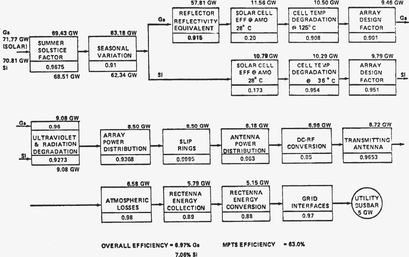
- An end-to-end efficiency chain from 70–72 GW of intercepted sunlight to 5 GW at the utility busbar, about 7 percent overall, with a 63 percent microwave link (Fig. 5, p. 13).
- A microwave design set by two limits, 22 kW/m² of waste heat in the transmitter and 23 mW/cm² in the ionosphere, giving a 10-dB tapered 1 km antenna and a 10 km rectenna (pp. 25–29).
- A mass statement of 34 and 51 million kg for the two options, including 25 percent contingency (Table 1, p. 48).
- A transportation fleet and construction scenario for building two satellites a year: a 424-tonne-payload reusable heavy lifter, electric cargo tugs, chemical crew transfer, and 375 or 225 heavy-lift flights per pair of satellites (pp. 47–75).
I. Summarypp. 1–2
The reference concept came mostly from two parallel but independent system definition studies. Boeing worked for Johnson Space Center (JSC) and Rockwell for Marshall Space Flight Center (MSFC). Their concepts agreed on some major elements and differed sharply on others. To meet the milestone with essentially a single concept, NASA built a third system from elements of both (p. 1).
All the supporting numbers assume two 5 GW satellites a year for 30 years: the first in service in 2000, and 10 GW added each year until 2030. The satellite is a planar array of about 55 km² on a graphite-fibre-reinforced thermoplastic structure, with a 1 km phased-array antenna at one end. It uses klystron amplifiers and slotted-waveguide radiators. Each satellite is built in geosynchronous orbit in six months, and its ground receiving station, the rectenna, is finished in the same time (pp. 1–2).
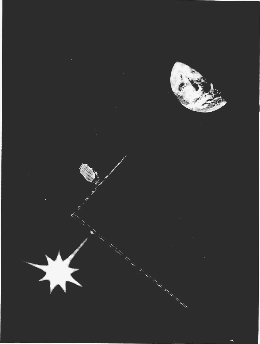
The program has two more big pieces: construction bases in orbit with launch and mission-control bases on the ground, and a fleet of vehicles to carry cargo and people up. These are a heavy-lift launch vehicle (HLLV), a personnel launch vehicle (PLV), a cargo orbit transfer vehicle (COTV) and a personnel orbit transfer vehicle (POTV). The launch site is Kennedy Space Center, pending further study (p. 2).
II. Introductionpp. 4–9
Under the joint program plan (DOE/ET-0034, February 1978), NASA does system definition, and DOE evaluates health, safety and environmental factors, economics, and international and institutional issues, and compares the concept with other future power sources. The milestones are a baseline concept in October 1978, preliminary recommendations in May 1979, updated ones in January 1980 and final ones in June 1980. The report says Reference System rather than baseline because the design is still immature (p. 4).
It is recognized that the Reference System lacks maturity as reported herein.II. Introduction, p. 4
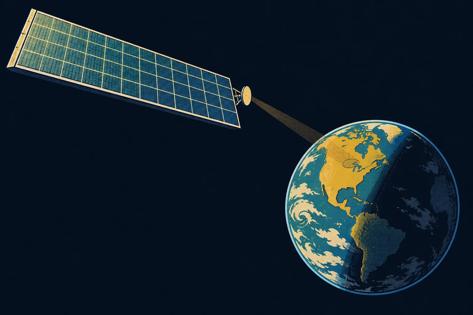
The concept itself (Fig. 3) is a primary power source: generate electricity from sunlight in geosynchronous orbit, send it to Earth on focused microwave beams, and turn the beams back into electricity on the ground. It traces to Peter Glaser's article in Science of 22 November 1968 (p. 6).
Four alternatives are set aside, with reasons (pp. 8–9):
- Orbiting nuclear reactors would be more compact but heavier and more complex than solar power, with significant open safety and environmental questions.
- Power relay satellites, which reflect power beamed up from the ground, move energy over long distances but are not a primary source.
- Orbiting mirrors: from geosynchronous orbit the smallest spot on Earth would be about 330 km across. Lit continuously at about one Sun, it would warm to about 150 °F. Low-orbit mirrors would not stay over one site, and clouds would block them.
- Laser transmission has much lower efficiency and much higher atmospheric losses than microwaves.
Building satellites from lunar material, where gravity is one-sixth of Earth's, is noted as promising but would need mining, manufacturing and launch facilities on the Moon. The program therefore assumes terrestrial materials and geosynchronous deployment (p. 9).
III. Reference System Descriptionpp. 10–78
This part describes the system that came out of the Boeing and Rockwell studies. The report stresses that it is preliminary and incomplete in detail in some areas (p. 10).
A. Guidelines and Assumptionsp. 10
- Operational date 2000; two 5 GW systems a year, 300 GW total for costing purposes.
- Every rectenna sized for 5 GW. Geosynchronous orbit. Operating frequency 2.45 GHz.
- Microwave power density no more than 23 mW/cm² at the rectenna centre and 1 mW/cm² at its edge.
- All materials from Earth. A 30-year life, with no salvage value or disposal cost.
- Zero launch failures. Technology available by 1990.
- No cost margins; 1977 dollars; a 25 percent weight-growth factor reflected in costs.
B. System Overviewpp. 10–16
The system is sized for 5 GW of DC power into a conventional grid. It has one antenna, at one end, transmitting to one rectenna. The array is planar and built from graphite composite. Its size is dictated primarily by the efficiency chain (p. 11): with about 7 percent overall efficiency, 5 GW at the busbar needs about 70 GW of intercepted sunlight.
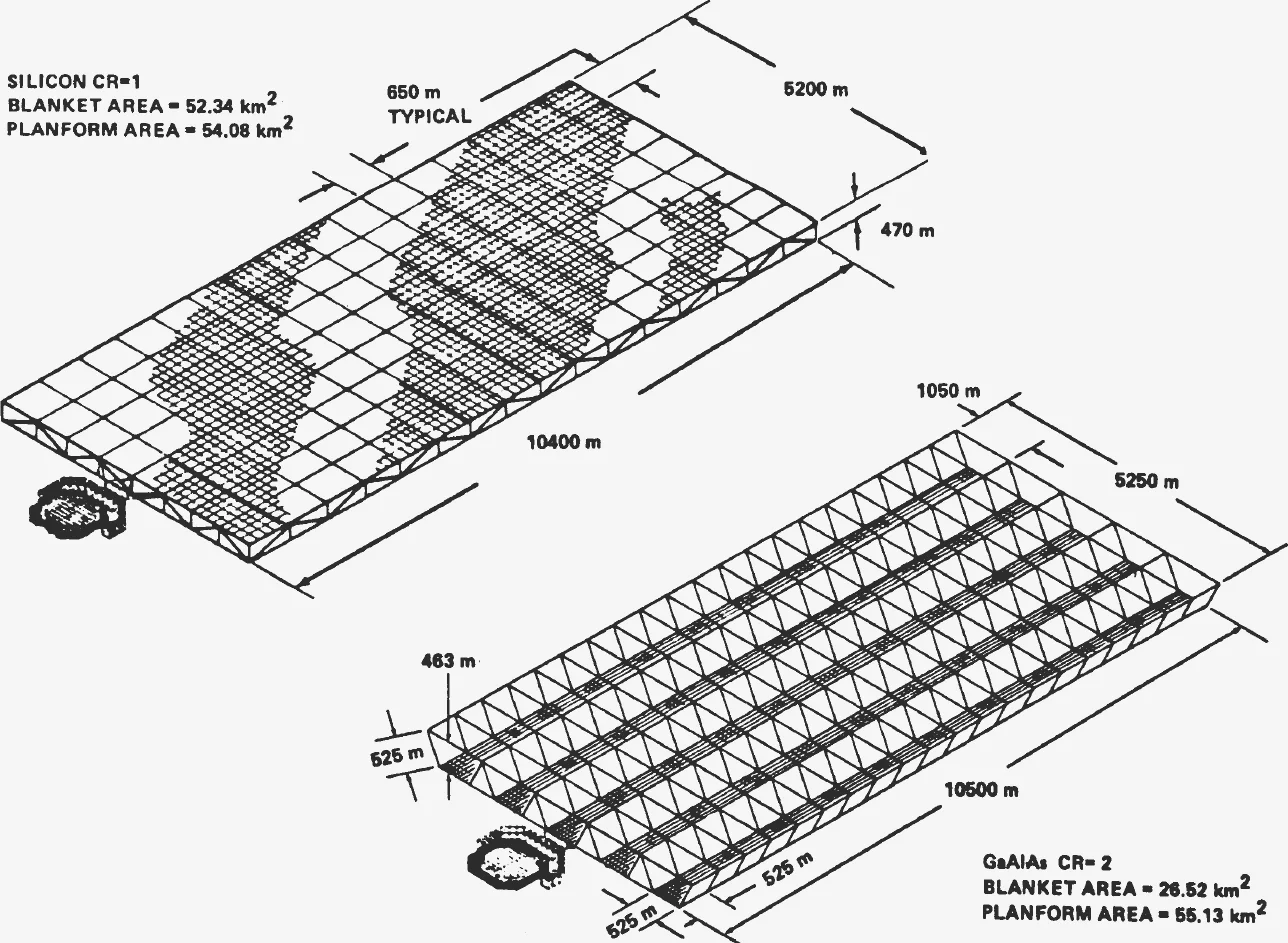
The GaAlAs option has five troughs: 26.52 km² of cell blanket, 53.04 km² of reflector and a planform of 55.13 km². The silicon option uses no concentration: 52.34 km² of blanket on a 54.08 km² planform. Either way the satellite flies with the antenna's main rotation axis perpendicular to the orbit plane (p. 11). The planforms are simply length times width: 10.4 × 5.2 = 54.08 km² and 10.5 × 5.25 = 55.13 km².
The quoted efficiency is a worst case. It includes the summer-solstice factor (0.9675), the seasonal variation (0.91) and end-of-life cell efficiency after annealing. For GaAlAs, the reflectors are 0.83 reflective at end of life, but only half the intercepted light reaches the cells by reflection, so the equivalent factor is (p. 11). Each element's factor multiplies:
is each element's efficiency from Fig. 5 and the collecting area. The report's inputs (70.81 GW for silicon, 71.77 GW for GaAlAs) equal the silicon blanket area and the GaAlAs reflector area times W/m², the solar constant implied by those figures.
- Season
- Solar array
- Satellite power and transmitter
- Atmosphere, rectenna and grid
- Sunlight in
- 71.77GW
- DC to grid
- 5.00GW
- Overall
- 6.97%
- Microwave link
- 63%
| Item | GaAlAs (CR = 2) | Silicon (CR = 1) |
|---|---|---|
| Generation at utility interface | 5 GW | 5 GW |
| Overall dimensions | 5.3 × 10.4 km | 5.3 × 10.4 km |
| Satellite mass | 34 × 10⁶ kg | 51 × 10⁶ kg |
| Structure | Graphite composite | Graphite composite |
| Construction location | GEO | GEO |
| Earth to LEO, cargo | Vertical take-off, winged, 2-stage (424,000 kg) | same |
| Earth to LEO, personnel | Modified Shuttle (75) | same |
| LEO to GEO, cargo / personnel | Dedicated electric OTV / 2-stage LOX–LH₂ (75) | same |
| Antennas · DC–RF converter · frequency | 1 · klystron · 2.45 GHz | same |
| Rectenna | 10 × 13 km | 10 × 13 km |
| Rectenna power density, centre / edge | 23 / 1 mW/cm² | same |
The rectenna has 78.5 km² of active panel area, exactly a circle 10 km across (). Construction crews are 555 for silicon (480 in GEO, 75 in LEO) and 715 for GaAlAs (680 in GEO, 35 in LEO) (pp. 11, 14).
C. Solar Cells and Blanketspp. 14–17
Both cell types are carried as reference options. Each makes a different bet on how to survive 30 years of radiation (pp. 14, 17):
| GaAlAs, CR = 2 | Silicon, CR = 1 | |
|---|---|---|
| Cell | 5 µm GaAs with a 0.03–0.05 µm GaAlAs window | 50 µm single-crystal silicon, both contacts on the back |
| Efficiency, AM0 at 28 °C | 20 % | 17.3 % (beginning of life) |
| Operating temperature and efficiency | 125 °C, 18.2 % | 36.5 °C, 16.5 % |
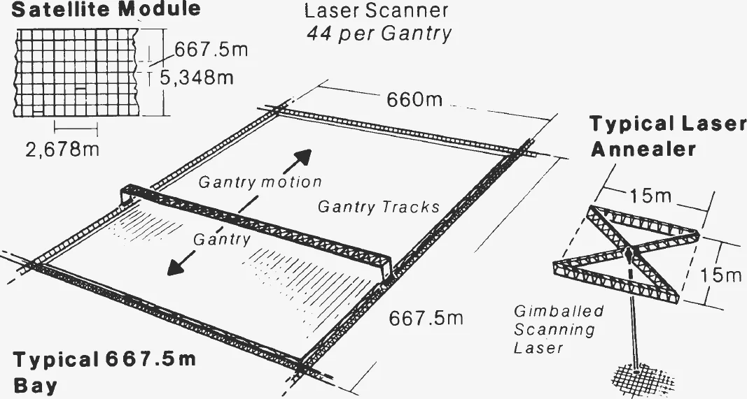
| Radiation recovery | Self-annealing at 125 °C | Laser annealing in place, cells heated to 500 °C |
| Blanket | 25 µm Kapton; 20 µm sapphire substrate doubles as cover; 0.252 kg/m² | Borosilicate glass bonded front and back; 12.5 µm silver-plated copper interconnects |
| Concentrator | 12.5 µm aluminised Kapton, 60° V-trough; reflectivity 0.9 new, 0.83 at end of life; 0.018 kg/m² | none |
| Projected blanket cost | $71/m² | $35/m² |
The operating-temperature efficiencies correspond to the cell-temperature factors in Fig. 5: 18.2/20 ≈ 0.91 and 16.5/17.3 ≈ 0.954.
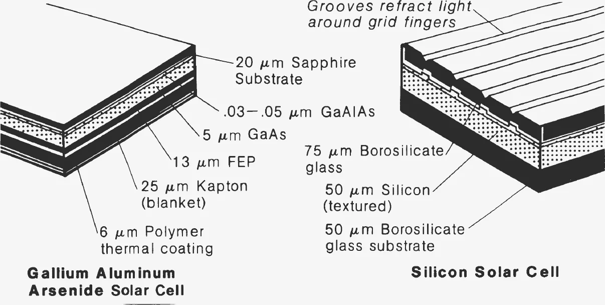
At the stated densities the GaAlAs blanket comes to about km² ≈ 6.7 million kg and the reflectors to km² ≈ 0.955 million kg, the figures that appear in the mass statement (Table 1). Appendix A notes that with concentration the gallium system has a cost advantage, while without it silicon would be competitive; because of this close competition both stay as candidates (p. A-13).
D. Solar Array and Structurepp. 17–19
Blankets go up in rolled or folded modules and are wired in series and parallel to reach 40 to 45 kV. GaAlAs reflector panels are pleated like an accordion, rolled for launch, and hung from the structure on catenary cables. The primary structure for both the array and the antenna is an open truss of graphite-fibre-reinforced thermoplastic, with beams designed for automatic fabrication in space (p. 19).
E–G. Power Distribution, Rotary Joint and Attitude Controlpp. 19–25
These three short sections are merged here. The array is split into switchable power sectors, so any sector can be isolated for annealing or repair. Voltage is held by switching groups of cell strings on and off. On the antenna, DC–DC converters and switchgear feed the klystrons, and about 12 MWh of batteries carry the antenna through eclipses and shutdowns (pp. 19, 22).
Power crosses to the antenna through slip rings and brushes in a rotary joint. A 350 m mechanical turntable turns the antenna yoke once a day. The antenna hangs in the yoke on a compliant joint and is aimed by control moment gyros on its own structure (p. 22).
Attitude control for the GaAlAs satellite uses 64 argon ion thrusters, about 36 of them operating at once, in four locations; this allows for annual maintenance, 5,000-hour grid life and a five-year mean time between failures. Each thruster gives 13 N at a specific impulse of 13,000 s, draws 1,275 kW, has a 1 m aperture and weighs 120 kg. The system averages 34 MW (pp. 22–25, Fig. 13). The satellite flies with its long axis perpendicular to the orbit plane.
H. Microwave Power Transmission Systempp. 25–46
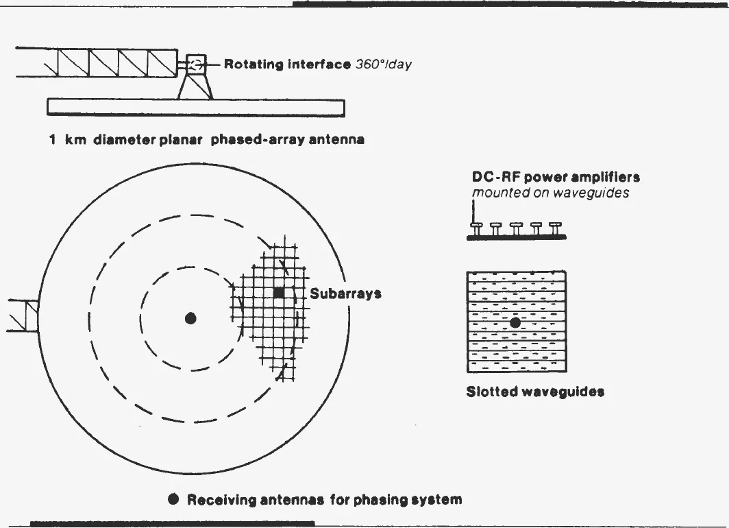
DC-to-RF converters feed a 1 km phased array with a 10-decibel Gaussian taper: the power density falls by a factor of ten from centre to edge. The antenna is built from 7,220 subarrays, each about 10 m square, with slotted aluminium waveguides on the front and the power tubes on the back. Every subarray has its own receiver and phasing electronics, which lock onto a pilot beam sent up from the rectenna. The subarrays add into one coherent beam focused on the rectenna centre. About 88 percent of its energy falls within 5 km of boresight, and the beam is 1.2 arc-minutes wide (p. 25).
Microwave system parameters and sizing considerationspp. 25–29
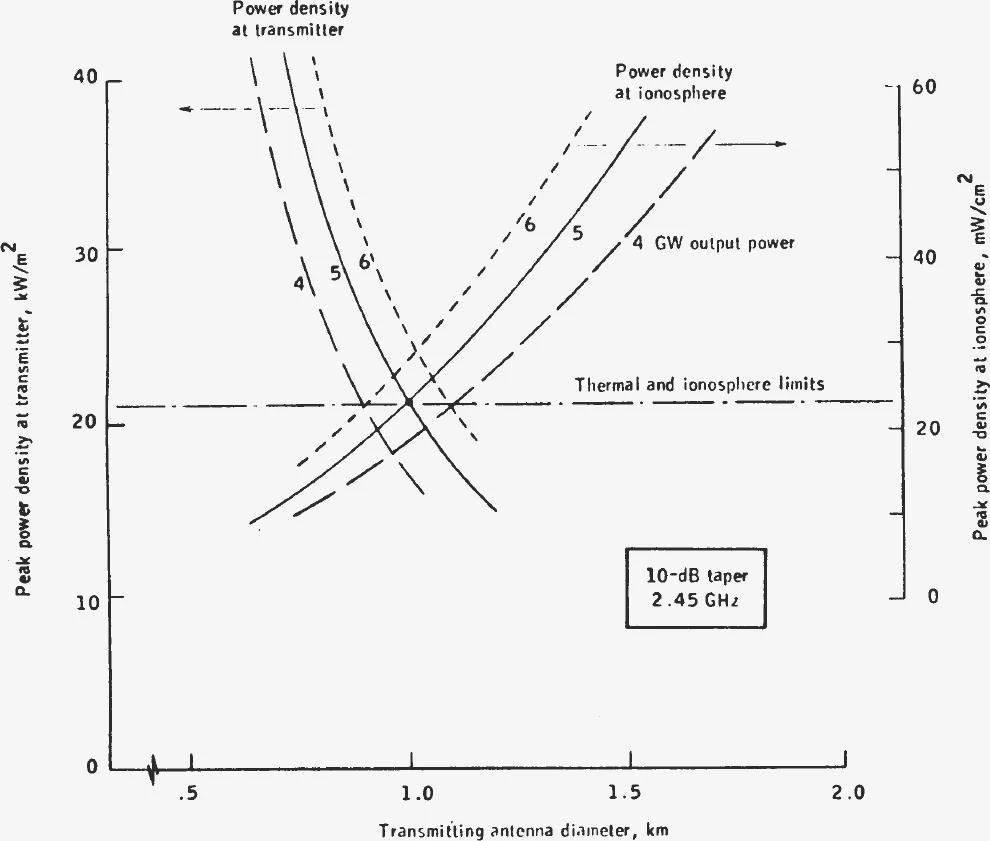
Three things set the power per antenna: the 22 kW/m² of waste heat the transmitter can shed, the 23 mW/cm² peak density the ionosphere is thought to tolerate, and the efficiency of the link, chiefly how much RF lands on the rectenna (pp. 25, 29). The ionospheric limit comes from theory. Above it, thermal self-focusing in the F region (200–300 km) and thermal runaway in the D region (100 km) could disturb HF and VHF communication and VLF navigation, and add phase jitter to the pilot beam (p. 29).
(which is a theoretical number, not yet verified by experiments)On the 23 mW/cm² threshold, p. 29
| Parameter | Value |
|---|---|
| Frequency | 2.45 GHz |
| Output to grid · transmit array diameter | 5 GW · 1 km |
| Power radiated · link efficiency | 6.72 GW · 63 % |
| Illumination | 10-step truncated Gaussian, 10 dB edge taper |
| Error budget | 10° rms phase per subarray; 2° mean phase at array edge; ±1 dB amplitude; 2 % of tubes failed |
| Mechanical alignment | ±3 arc-min, grating lobes ≤ 0.01 mW/cm² |
| Subarrays | 7,220 of 108 m² |
| Density at transmitter, centre / edge | 22 / 2.4 kW/m² |
| Density at rectenna, centre / edge | 23 / 1 mW/cm² |
| First sidelobe | 0.08 mW/cm², about 9 km from centre |
| Grating lobes | ≤ 0.01 mW/cm², every 440 km |
| Out-of-band noise | below CCIR −180 dBW/m²/Hz above 25° arrival |
| Converter · radiator · material | Klystron · slotted waveguide · aluminium |
Antenna characteristicspp. 29–30
The primary structure is an octagonal open truss 130 m deep and over 1,000 m across. A deployable cubic truss 9.93 m deep holds the subarrays. Of the illumination functions studied, with phase and amplitude errors and failed elements included, the 10-dB Gaussian taper performed best overall within the density limits at both ends (p. 29).
The taper is built in ten steps: 36 tubes per subarray at the centre, falling to 4 at the edge, for 101,552 tubes of 70 kW each. A 50 kW alternative would need about 140,000, from 50 per subarray at the centre down to 6 (p. 30).
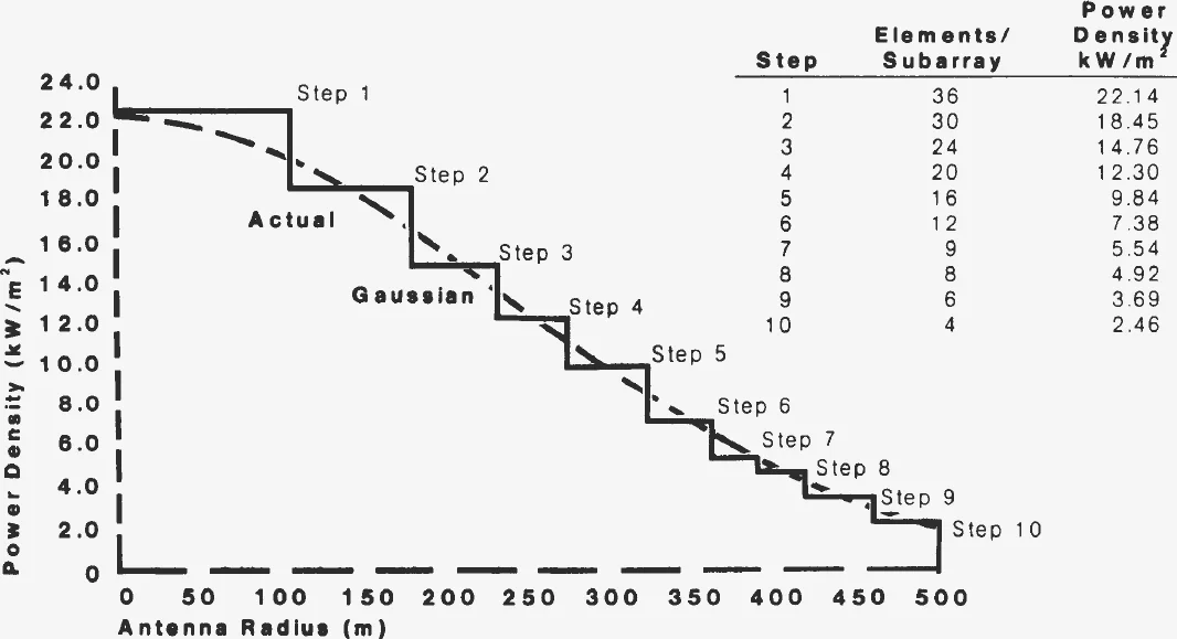
| Step | Outer radius, m | Subarrays | Elements / subarray | Tubes | kW/m² |
|---|---|---|---|---|---|
| 1 | 93.9 | 276 | 36 | 9,936 | 22.14 |
| 2 | 177.3 | 632 | 30 | 18,960 | 18.45 |
| 3 | 229.5 | 644 | 24 | 15,458 | 14.76 |
| 4 | 271.2 | 628 | 20 | 12,560 | 12.30 |
| 5 | 323.3 | 784 | 16 | 12,544 | 9.84 |
| 6 | 365.1 | 900 | 12 | 10,800 | 7.38 |
| 7 | 396.3 | 664 | 9 | 5,976 | 5.54 |
| 8 | 417.2 | 612 | 8 | 4,896 | 4.92 |
| 9 | 458.9 | 1052 | 6 | 6,312 | 3.69 |
| 10 | 500.6 | 1028 | 4 | 4,112 | 2.46 |
| Total | 7,220 | 101,552 |
Radii from Fig. 17, elements per subarray and power density from Fig. 16, subarray and tube counts from Fig. 17.
The beam at the rectennapp. 30–37
Antenna errors give a wider, weaker main beam and higher sidelobes. Only part of the main lobe is collected; the sidelobes spread over a huge area at densities too low to be worth collecting (p. 30). The peaks are 23 mW/cm² at boresight, 1 mW/cm² at the rectenna edge and 0.08 mW/cm² in the first sidelobe, two orders of magnitude below the U.S. standard of 10 mW/cm² (p. 30).
For a circular aperture of uniform rings at range , the far-field density on the ground at distance from boresight is
and are each step's density and outer radius (Figs. 16–17), cm at 2.45 GHz, km (App. A, p. A-2), and is the Bessel function. At the centre this reduces to , where is the taper's aperture efficiency, worked out from the Fig. 16 densities.
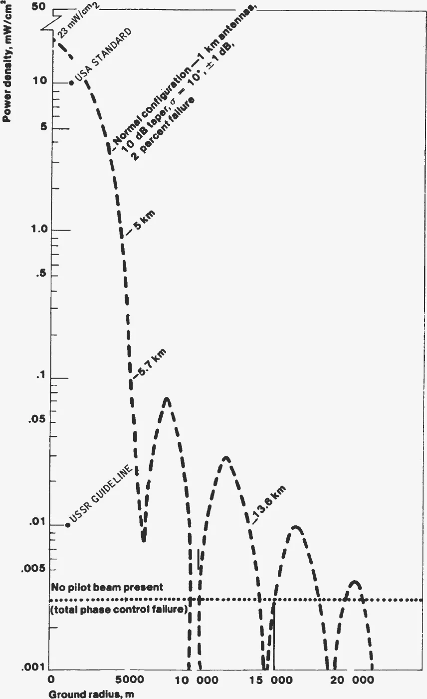
- Ground power density
- Report's printed values (Fig. 15)
- Inside the rectenna (dashed: edge)
- U.S. exposure standard 10, USSR guideline 0.01 mW/cm²
- Beam defocused (no pilot signal) 0.003 mW/cm²
- Centre
- 23.2mW/cm²
- At edge
- 0.82mW/cm²
- Captured
- 90.1%
- 1st sidelobe
- 0.083@ 8.0 km
If phase control fails completely, for example if the pilot transmitter shuts off, the subarrays lose phase and the beam spreads out. The peak falls to 0.003 mW/cm², which the report calls a fail-safe feature, below the USSR guideline. Sensors near the rectenna would also detect large changes and shut the antenna down (p. 30).
Why the fail-safe works: with random phases the subarrays add in power rather than in field, so the whole 6.7 GW is spread as if by a single 108 m² subarray () instead of the full 1 km aperture.
Far sidelobes from one satellite are three to four orders of magnitude below 0.01 mW/cm². Even 200 satellites would stay one to two orders below it. The downlink sits in the 2,400–2,500 MHz industrial, medical and scientific band, which some eastern European countries do not recognise (p. 34).
Grating lobes repeat every 440 km on the ground. They come from the regular subarray spacing and depend on mechanical misalignment; uniquely, they stay put while their strength varies, because of the retrodirective phasing. Keeping them under 0.01 mW/cm² requires antenna tilt under 1 arc-minute and random subarray tilts under 3 (pp. 34–37). Their spacing is for subarray pitch m; at a slant range of about 37,400 km, typical of a mid-latitude rectenna, that is 440 km.
Close to the antenna the beam has not formed yet. On the axis, density peaks at about 32 kW/m² some 1,600 km out (p. 37, Fig. 23).
Rectenna characteristicspp. 37–43
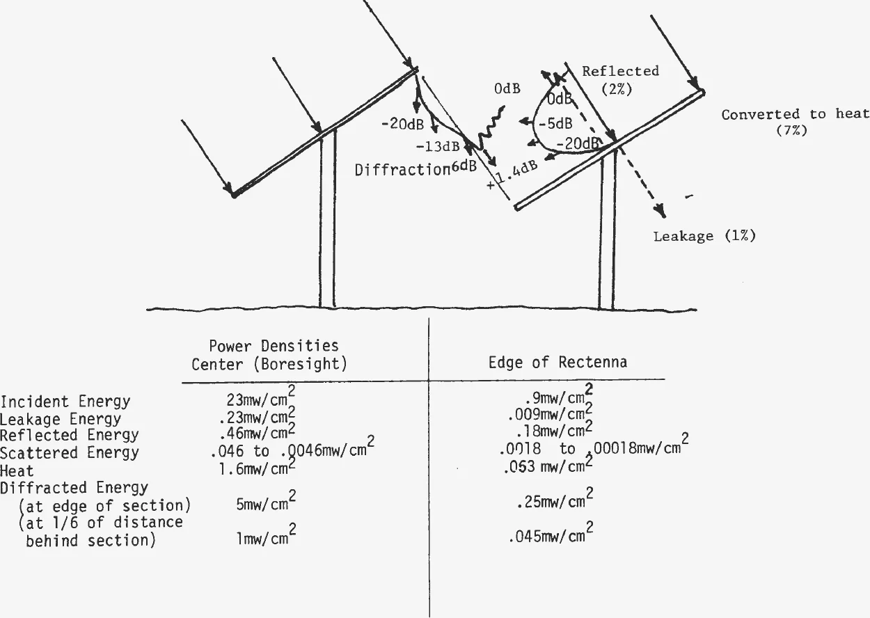
The rectenna is a field of half-wave dipoles, each feeding a Schottky-barrier diode through a two-stage low-pass filter that suppresses harmonics and matches impedance. To save money it is built as rows of serrated panels square to the incoming beam rather than a continuous surface. Each panel has a steel-mesh ground plane of 75–80 percent optical transparency on steel framing and concrete footings, with aluminium collector wiring (p. 37). The total active panel area is 78.5 km² (p. 41).
Of the incident power, about 98 percent is collected by the dipoles and 2 percent reflected, upward and toward the southern horizon. About 1 percent leaks through the mesh, and about 7 percent becomes heat in the elements and diodes. Diode harmonics are −25, −40 and −70 dB for the second, third and fourth (pp. 41–43).
The beam arrives at a slant, so its circular cross-section lands as an ellipse. A 10 × 13 km rectenna (Fig. 7) implies a stretch of 1.3, which corresponds to a site near 35° latitude below a satellite on the same meridian (from the geometry of geostationary orbit). The 78.5 km² is the area measured square to the beam.
Microwave system efficiency, phase control and RFIpp. 43–46
From DC at the rotary joint to DC out of the rectenna, the link is 63 percent efficient (p. 43):
Report Fig. 25 (p. 44). The antenna factor is 0.985 for resistive loss times 0.98 for pointing and subarray and waveguide tolerances, for a 10 km rectenna with the Fig. 15 error budget.
The phase control system has four parts: a phase-lock loop around every tube; a pilot beam with double sidebands placed symmetrically about the downlink frequency, so there is no beam squint, offset by more than 10 MHz (the ionosphere's maximum plasma frequency); coded pilot signals, so each satellite answers only its own rectenna and resists interference; and ground sensors with a command link for safety. Whether to conjugate phase at each subarray or at each tube was still being traded (pp. 43–45).
Radio interference comes mainly from the tubes, through sidelobes and grating lobes, noise near the carrier and harmonics. The phase-lock loops and multi-cavity klystrons, filtering 24 dB per octave out of band, keep spurious noise under the CCIR limit of −180 dBW/m²/Hz (pp. 45–46, Fig. 26).
I. Mass Statementpp. 47–48
Mass falls into three parts: solar array, antenna, and the interface between them (rotary joint, slip rings, yoke). The antenna is the same for both options and is dominated by the transmitter subarrays with their klystrons and waveguides. Concentration halves the GaAlAs blanket area and with it most of the mass difference (p. 47).
| Subsystem | GaAlAs CR = 2 | Silicon CR = 1 |
|---|---|---|
| Solar array | 13.798 | 27.258 |
| Primary structure | 4.172 | 3.388 |
| Secondary structure | 0.581 | 0.436 |
| Solar blankets | 6.696 | 22.051 |
| Concentrators | 0.955 | — |
| Power distribution & conditioning | 1.144 | 1.134 |
| Information management & control | 0.050 | 0.050 |
| Attitude control & stationkeeping | 0.200 | 0.200 |
| Antenna | 13.382 | 13.382 |
| Primary / secondary structure | 0.250 / 0.786 | 0.250 / 0.786 |
| Transmitter subarrays | 7.178 | 7.178 |
| Power distribution & conditioning | 2.189 | 2.189 |
| Thermal control | 2.222 | 2.222 |
| Information management & control | 0.630 | 0.630 |
| Attitude control | 0.128 | 0.128 |
| Array/antenna interfaces | 0.147 | 0.147 |
| Subtotal | 27.327 | 40.787 |
| Contingency (25 %) | 6.832 | 10.197 |
| Total | 34.159 | 50.984 |
Per kilowatt delivered, the totals are about 6.8 kg/kW for GaAlAs and 10.2 kg/kW for silicon.
J. Space Transportationpp. 47–58
The fleet is dedicated to the program and designed for minimum total cost, with energy use, environmental impact and critical materials kept low. Cargo goes up on the HLLV and people on the PLV. Between low orbit and geosynchronous orbit, cargo rides the COTV and people the POTV (pp. 47, 49).
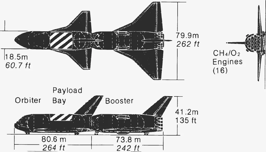
| Vehicle | Description | Key numbers |
|---|---|---|
| HLLV | Two-stage, vertical take-off, horizontal landing, fully reusable | GLOW 11,040 t; 424 t to LEO; booster 16 × 9.79 MN (CH₄/O₂), orbiter 14 × 2.09 MN (SSME); booster lands at 934 t, orbiter at 453 t with 63.5 t returned |
| PLV | Shuttle orbiter with a liquid fly-back booster and a passenger module | 75 passengers; smaller external tank with 546 t of propellant versus 715 t today |
| POTV | Two-stage LOX–LH₂, common stages | 890 t at start of burn; 151 t up (160 people, 480 man-months of supplies, crew of 2), 55 t down |
| COTV, GaAlAs | Self-annealing GaAlAs array, CR 2; 259 ion thrusters, 100 cm, Isp 13,000 s, argon | 3,469 t payload; 572 t dry + 25 %; 185 t propellant up; LEO–GEO 133 days, round trip < 180 days |
| COTV, silicon | Planar silicon array; four modules of 296 ion thrusters, 120 cm, Isp 7,000 s, argon | 4,000 t payload; 965 t dry + 25 %; 835 t propellant up; round trip about 160 days |
Total COTV mass in LEO, with payload and propellant: 4,396 t (GaAlAs) and 6,191 t (silicon). The HLLV payload is 3.8 % of its lift-off weight.
K. Natural Resourcespp. 58–64
Table 4 lists the materials, in tonnes, for the satellite, rectenna and every vehicle, split into what is specific to the silicon program, what is shared, and what is specific to GaAlAs. Table 5 totals them for the first satellite, which carries the construction bases and the COTV fleet, and for each later year of two satellites. The GaAlAs program's construction bases appear only as total-mass estimates, still under study (pp. 58, 64).
L. Operationspp. 64–76
Each satellite needs mass production on a new scale: about solar cells, klystrons and dipoles. Launches burn about t of hydrocarbon propellant a year, and options from coal processing to rectenna-powered electrolysis were under study. Packaging matters: densities range from 12 kg/m³ for antenna subarray elements to about 2,500 kg/m³ for conductors, so loads are mixed to fill each launch (pp. 64–66).
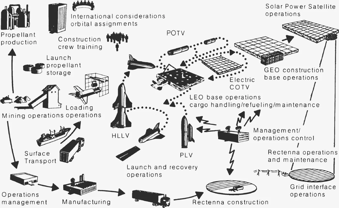
Startup. Before any satellite is built there are two years of preparation. For silicon: six months to build the LEO base, three for the first COTV, three more for the second and third, and a year for the rest of the fleet; the first COTVs carry up the GEO base, which takes nine months. For GaAlAs the GEO base is built in LEO first, builds the COTVs there, and is then towed up by two of them (p. 69).
Steady state. All the material for one satellite reaches LEO in six months, rides COTVs for six months to GEO, and is assembled during a six-month arrival window. The sequence for any pair takes 18 months, but once it is running two satellites come off the line each year (p. 69).
| Silicon | GaAlAs | |
|---|---|---|
| SPS mass | 50,984 t | 34,159 t |
| HLLV flights (424 t each) | 375 | 225 |
| PLV flights (75 people) | 30 | 38 |
| COTV flights | 30 (4,000 t) | 22 (3,500 t) |
| POTV flights (160 people, 400 t) | 12 | 17 |
| Packing factor, hardware / propellant | 85 % / 95 % | 95 % / 95 % |
| People at LEO staging base / GEO | 75 / 480 | 35 / 680 |
| HLLV boosters | HLLV orbiters | PLV | COTV | POTV | |
|---|---|---|---|---|---|
| Startup | 2 (1) | 3 (1) | 2 | 3 (2) | 2 (1) |
| Added for two satellites a year | 2 (2) | 2 (2) | — | 20 (8) | — |
| Total | 4 (3) | 5 (3) | 2 | 23 (9) | 2 (1) |
Silicon first; GaAlAs in parentheses. The GaAlAs program needs fewer COTVs because of its different COTV design and trip times, lighter satellite and better packing (p. 73).
In commercial service, output varies with season, time of day and orbit, and eclipses cause shutdowns, so ground plants must be able to throttle to follow demand. With about klystrons failing at random and blanket sections occasionally replaced after meteoroid damage, each satellite needs 5 to 20 people in GEO, probably based at the construction base (p. 73). Program headquarters, launch control, the LEO and GEO bases, and a control unit at each rectenna make up the management concept (p. 76).
M. Costsp. 76
This section is two sentences long. Costs had been estimated, but they were held for the DOE Comparative Assessment Study and are not given here (p. 76).
IV. Technology Summarypp. 79–82
The report lists the critical questions on which feasibility rests, in seven areas (pp. 79–81):
- Microwave transmission: DC–RF amplifiers, phase control, subarray design with an integrated systems test, and rectenna components and construction.
- Solar arrays: low-cost automated blanket production, long-term radiation, UV and plasma effects at high voltage, annealing methods, and reflectors.
- Power distribution: spacecraft charging, 40–50 kV DC switchgear and cable insulation, 30-year slip rings, and power processing for electric propulsion.
- Structures and control of large lightweight systems; materials stability in GEO and LEO.
- Construction: beam builders, crane-manipulators and remote work stations, and ways to install blankets, conductors and subarrays.
- Space transportation: electric propulsion, large long-life liquid engines for the HLLV, and handling fluids in orbit.
Alternatives to reduce risk: amplitrons, magnetrons or solid-state amplifiers instead of klystrons; amorphous silicon, cadmium sulfide or other cheap cells, or potassium Rankine and Brayton heat engines instead of photovoltaics; aluminium structure; and a single-stage-to-orbit launcher instead of the two-stage HLLV (p. 82).
V. Documentation Summarypp. 83–87
Forty-seven references, grouped by subject and in date order within each group. They run from Glaser's 1968 paper and the 1976 JSC and MSFC in-house evaluations, through the Boeing and Rockwell system definition reports and W. C. Brown's Raytheon microwave power transmission work, to studies of ionospheric heating, rectenna structures, microwave bioeffects and economic, legal and political questions. Some are marked for restricted distribution (pp. 83–87).
Appendices A and Bpp. A-1 ff., B-1 ff.
Appendix A traces the trade studies behind each choice, from early concepts to the reference system. Appendix B describes the independent Boeing and Rockwell systems. A few Appendix A results explain the shape of the reference design (pp. A-2 to A-10):
- Orbit: geostationary, at 35,800 km with zero inclination and eccentricity. Inclined orbits would sweep the beam's angle at the rectenna each day; a 7.3° orbit would avoid lunar and solar perturbations that otherwise swing the inclination between zero and 15° over years. An eccentric orbit would raise the risk of collision with other synchronous satellites.
- Attitude: the array is held perpendicular to the orbit plane all year instead of tracking the Sun's 23.4° seasonal swing. This removes the annual gravity-gradient torque and saves propellant, at a maximum power loss of about 8 percent.
- Eclipses: daily shutdowns around local midnight for about six weeks each spring and autumn, lasting up to about 75 minutes.
- Sizing: the transmitter heat limit falls with antenna diameter and the ionospheric density rises with it, so together they fix both the maximum output and the antenna size.
is the peak density in the transmitter, its peak-to-average ratio for the 10-dB taper, the peak at the beam centre, the main-beam factor (taper, error budget and atmosphere), and the two limits. With 22 kW/m² and 23 mW/cm² this gives about 6.7 GW radiated, or 5 GW at the busbar, from a 1 km antenna: the reference design.
- Heat in transmitter ÷ thermal limit
- Beam centre at ionosphere ÷ ionosphere limit
- Diameters meeting both limits
- Selected diameter
- Transmitter
- 22.1kW/m²
- Beam centre
- 23.0mW/cm²
- Best output
- 4.99GW @ 1.00 km
- Rectenna
- 10.0km across
Assumptions and open questions
Key assumptions
- Program ground rules (p. 10): two 5 GW satellites a year for 30 years starting in 2000, zero launch failures, technology available by 1990, no cost margins, and no salvage or disposal cost. The fleet, crew and materials figures are built on these.
- The ionospheric limit. A peak of 23 mW/cm² at the beam centre sets the antenna size, the rectenna size and the power per satellite. The report describes it as a theoretical threshold awaiting experiment (p. 29).
- The transmitter heat limit of 22 kW/m² (21 kW/m² in Appendix A) reflects how much klystron waste heat the antenna can reject.
- Worst-case rating. The 5 GW is set at summer solstice with end-of-life cells (p. 11). Eclipses of up to about 75 minutes around local midnight, for some six weeks each spring and autumn, are outside the rating (p. A-10).
- Antenna tolerances of 10° rms phase, ±1 dB amplitude and 2 percent failed tubes (Fig. 15) underlie the beam pattern, the 88 percent beam capture and the 63 percent link efficiency.
- Earth materials and geostationary assembly throughout, with lunar materials and other orbits left for later study (p. 9).
Where further work would help
The two microwave limits. Because transmitter density scales as and beam-centre density as , the largest output per satellite scales as and the antenna diameter as (see the sizing figure). Measurements of how the ionosphere responds near 23 mW/cm², which the report notes were under way both theoretically and experimentally (p. 29), and of achievable antenna heat rejection would show how far the 5 GW, 1 km, 10 km combination can move.
Building and holding the array's tolerances. The beam shape, sidelobes and grating lobes depend on the phase, amplitude, failure and alignment budgets of Fig. 15 and on the open choice between phase conjugation at each subarray or at each tube (p. 43). Hardware tests of subarrays and of the pilot-beam phasing system, which head the report's list of critical questions (p. 80), would show how well the design holds over a 1 km structure.
Thirty years in orbit. The end-of-life efficiencies assume annealing recovers radiation damage: self-annealing at 125 °C for GaAlAs, laser annealing for silicon. Long-duration tests of blanket materials under radiation, UV and plasma at 40–50 kV, of 30-year slip rings, and of composite stability in GEO and LEO (pp. 80–81) would show whether these factors carry over the full design life.
Scale-up on the ground and in space. Each satellite needs about cells, klystrons and dipoles (p. 64), and the construction scenario depends on space fabrication, electric orbit transfer and a fully reusable heavy lifter that did not yet exist. Rectenna construction methods had not yet been worked out (p. 73). Demonstrations at intermediate scale would show how the timeline and fleet sizes extrapolate to two satellites a year.
Costs and siting. Cost estimates were held for DOE's comparative assessment (p. 76), and rectenna land use and latitude are left to later studies. Both are needed before the reference system can be compared with other power sources.
What happened next
- 1979
January: the report, dated October 1978, is published as DOE/ER-0023. The joint plan's next milestones are preliminary program recommendations in May 1979 and updated ones in January 1980.
- 1980
Apr 22–25: DOE and NASA hold the Solar Power Satellite Program Review at the University of Nebraska–Lincoln. The proceedings say the four-year program would conclude in the fall of 1980 with recommendations (NASA TM-84183).
- 1980
November: NASA's technical assessment summary report (NASA TM-58232) sums up the system definition work: the reference satellite and its subsystems, the orbital construction and maintenance bases, the space transportation system, the ground receiving station and the industrial facilities needed to build them.
- 1995
After a hiatus of about 15 years, NASA reexamines space solar power in its 1995–97 fresh look study, followed by a concept definition study in 1998 and the SSP Exploratory Research and Technology program in 1999–2000 (Howell & Mankins, NTRS 20000044328).
- 2001
NASA starts the SSP Technology Advanced Research and Development (STAR-Dev) program, aimed at technology for multi-megawatt to gigawatt-class systems and wireless power transmission (NTRS 20010019996).
- 2024
January: NASA's Office of Technology, Policy and Strategy reports that the 1970s and 1990s studies found such systems prohibitively expensive, citing a $1T then-year estimate for a 1970s technology demonstration. It finds that representative modern designs would still cost more than terrestrial alternatives, with launch the largest cost driver.
Sources
- Satellite Power System: Concept Development and Evaluation Program — Reference System Report, DOE/ER-0023 (1978) · NTRS record and scan
- The Final Proceedings of the DOE/NASA Solar Power Satellite Program Review, NASA TM-84183 (1980)
- Satellite Power System Concept Development and Evaluation Program, Vol. 1: Technical Assessment Summary Report, NASA TM-58232 (1980)
- Howell & Mankins, Preliminary Results From NASA's Space Solar Power Exploratory Research and Technology Program (2000)
- Howell, Mankins & Davis, Overview of NASA's Space Solar Power Technology Advanced Research and Development Program (2001)
- NASA Office of Technology, Policy and Strategy, Space-Based Solar Power (2024)
- NASA: New Study Updates NASA on Space-Based Solar Power