At a glance
- Category
- An engineering systems design study. Part tutorial (Chapters 2–4 and parts of 5–6 introduce exobiology and interstellar communication), part conceptual design with subsystem sizing and costing (Chapters 7–14). The Foreword describes it as roughly two to three man-years of effort, a very preliminary and rough set of estimates (p. 2).
- Context
- The 1971 NASA–ASEE Summer Faculty Fellowship Program in Engineering Systems Design, run jointly by Stanford and NASA Ames (p. 1). It builds on Cocconi and Morrison's 1959 suggestion of the hydrogen line, Frank Drake's 1960 Project Ozma search of two nearby stars, and engineering work on very large radio telescopes then in progress, notably NRAO's proposed Very Large Array and the Bonn 100-m dish (pp. 63–64, 69–70, 82).
- Contributions
- A reaffirmation that the microwave window, and especially its low-frequency end, is the best part of the spectrum for interstellar search (Foreword, p. v; Ch. 5).
- The identification of the water hole, the quiet band between the hydrogen line (1420 MHz) and the lowest hydroxyl line (1662 MHz), as a natural meeting place (p. 64).
- A data processing design able to search at least half of that band at once and detect coherent signals about 90 dB below the total noise in the band (p. v; Ch. 11).
- Designs for local-oscillator distribution, IF transmission and delay, and low-noise remotely tunable receivers that make an array of several square miles of collecting area practical (p. v; Chs. 9–10).
- A first estimate of the major costs of an expandable search system and programme (p. v; Ch. 7).
1. Introductionpp. 1–2
Each summer NASA funds faculty fellowship programmes with the American Society for Engineering Education. Project Cyclops was the 1971 engineering-design programme run jointly by Stanford University and Ames Research Center (p. 1). Its primary objective was to assess the hardware, manpower, time and funding needed to mount a realistic effort to detect extraterrestrial intelligent life, using present or near-term technology.
A realistic effort means one with a high probability of success. Because the density of communicative life, and hence the volume to be searched, is unknown, Cyclops is designed as the minimum system likely to be needed, then enlarged until success or until a better technique appears. It is a flexible expandable system, not a fixed one (p. 1).
The authors stress how preliminary the numbers are: the study is two to three man-years of work, a go/no-go cost estimate would take ten times that, and a final design a thousand times. They ask that planned radio-astronomy and deep-space facilities be judged without regard to the report (p. 2).
2. Life in the Universepp. 3–28
A long tutorial chapter traces the converging disciplines of astronomy, geochemistry and biochemistry: the origin of matter, stellar populations and lifetimes, the formation of planetary systems, atmospheric evolution, the origin and evolution of life, and the rise of intelligence and technology (pp. 3–24). Condensed here to its quantitative thread.
Good suns. Dole's ecosphere limits of 65–135 percent of Earth's insolation are quoted, along with a 66 percent chance that a planetary system has one planet favourably placed (p. 17). Stars hotter than about F4 live too briefly; for cooler stars the limit is tidal braking of a planet's rotation, which the authors place between K0 and K7 depending on how much tide is tolerable. All F, G and K main-sequence stars should be included, with G stars given priority (pp. 17–18).
Concatenated probabilities. The number of sites with advanced life is written as a product of selectivity factors, which leads to Drake's expression for the number of communicative civilizations in the Galaxy (pp. 25–26):
= mean rate of star formation; = fraction of stars with planets; = suitable planets per ecosphere; = fraction on which life starts; = fraction evolving intelligence; = fraction attempting communication; = longevity of the communicative phase, years.
With the very approximate and probably optimistic values /yr, , , , and , the product of the factors is one, so : the number of communicating races is about the number of years each spends communicating, the most uncertain factor of all (p. 26). Dividing by the number of stars gives the a priori probability that a star chosen at random hosts a communicative race, , with for well-chosen target stars (eq. 16, p. 26).
The probability of interstellar communication. If races search and radiate only sporadically, the search can be long. But if communication is already established, a feedback effect (after von Hoerner) keeps beacons running for very long times and contact may be far easier than expected: 100 to 10,000 stars might need to be searched, a day to four months of observing (p. 27).
3. Some Reasons for the Searchpp. 29–32
The chapter frames contact as an effort comparable to Apollo, justified on the assumption that humanity survives as an evolving species for a very long time (p. 29). Its sections cover the continuing adventure of exploration, bio-cosmology, the possibility of joining a galactic heritage, and the possible hazards of contact, grouped as invasion, exploitation, subversion and cultural shock (p. 31). The authors' opinion is that the benefits very probably outweigh the risks; detecting signals jeopardises nothing, and they ask that any decision to respond, or to radiate a long-range beacon, be debated at a national or international level first (p. 32).
4. Possible Methods of Contactpp. 33–36
Interstellar travel. A chemical rocket leaving the solar system at about would take 40,000 years to reach α Centauri (p. 33). Even the ideal photon rocket, with mass ratio
= coordinate distance travelled per unit of ship's proper time. Accelerating and stopping at both ends of a round trip needs .
needs for . A 1,000-ton ship would leave at 34,000 tons and annihilate 33,000 tons en route, releasing J, enough to run a 1000-MW beacon for over 30 million years (p. 34).
Probes and serendipity. Bracewell's idea of probes parked at other stars would need about of them to cover the likely stars within 1000 light-years, launched at one a day for some 3,000 years (p. 35). Dyson's suggestion of looking for the infrared excess of engineered planetary systems is examined and set aside, since excess infrared lacks the hallmark of intelligence (pp. 35–36).
Communication alternatives. Communication needs particles that are cheap per quantum, fast, easy to generate and capture, and unaffected by the interstellar medium. Photons win, and low-frequency photons above all: a 1420-MHz photon carries one ten-billionth the kinetic energy of an electron at half the speed of light (p. 36).
5. Communication by Electromagnetic Wavespp. 37–52
Antenna gain and the free space transmission lawpp. 37–38
A uniformly illuminated aperture of area has on-axis power gain, and half-power beamwidth,
= aperture diameter, = wavelength.
Power radiated with gain toward a receiving antenna of area at distance delivers
is the effective radiated power.
For fixed antenna areas transmission improves with frequency, but at fixed gain the moves to the numerator and favours low frequencies. Practical gain tops out near , a beam of about one arc-second, at both optical and microwave wavelengths. For signals not under our control, eqs. (4)–(5) are the right form (p. 38).
Noise in coherent receivers, detection and filteringpp. 38–41
An ideal coherent amplifier has noise power per hertz , usually expressed as a noise temperature :
= Planck's constant, = Boltzmann's constant, = frequency, = temperature of the source or field of view. The first term is black-body radiation in one mode; the second, spontaneous emission in the amplifier. At radio frequencies ; at optical frequencies .
With synchronous detection and a matched filter, the output peak signal-to-noise ratio depends only on received energy per pulse and noise spectral density: (eq. 12). Since energy can only grow with signal duration once power is limited, we would expect interstellar contact signals to be highly monochromatic (p. 39). In the search, before a signal is known, square-law (energy) detection must be used: at high signal levels it gives one-quarter the synchronous detector's signal-to-noise ratio, and below the noise the number of averaged samples must grow as the inverse square of the input ratio (pp. 40–41).
The microwave window and star noisepp. 41–43
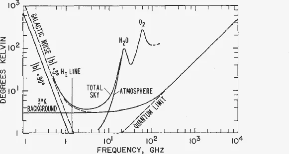
Three noise sources define a broad quiet region from roughly 1 to 100 GHz that would look nearly the same to observers anywhere in the solar neighbourhood: galactic synchrotron noise falling steeply with frequency, the 3 K cosmic background, and quantum noise rising as (p. 41). An Earth-like atmosphere adds water-vapour and oxygen lines at 22 and 60 GHz. The total sky temperature is about 4 K near the hydrogen line, with a minimum of about 3.6 K at twice that frequency, so the window from 1 to 10 GHz is clearly an attractive region for a ground-based receiver (p. 41).
Pointing at a star adds star noise. Weighting the field by the antenna pattern gives the increase in system temperature, which has the form of the transmission law with the star's projected area playing the transmitter (p. 42):
= effective temperature of the star at wavelength ; = receiving area; = range.
| λ, cm | T★ quiet, K | T★ active, K | ΔT quiet, K | ΔT active, K |
|---|---|---|---|---|
| 1 | 6,000 | 7,000 | 0.8 | 0.93 |
| 3.16 | 1.6 × 10⁴ | 6 × 10⁴ | 0.214 | 0.8 |
| 10 | 5 × 10⁴ | 1.5 × 10⁶ | 0.067 | 2 |
| 31.6 | 1.7 × 10⁵ | 4 × 10⁷ | 0.023 | 5.3 |
| 100 | 5 × 10⁵ | 8 × 10⁸ | 0.0067 | 10.7 |
Solar temperatures taken from Kraus. Star noise is detectable but not a serious problem for antennas up to 10 km and stars beyond 10 light-years unless they are more active than the Sun (p. 42).
Range limits and comparison of several interstellar linkspp. 43–51
For comparison the range limit is defined as the range at which a coherent receiver sees unity signal-to-noise ratio, and every other system is held to the same bit error rate, 0.07865, which is what a synchronous detector gives at unity input signal-to-noise (pp. 43–44). With a clear circular receiving aperture and overall efficiency , the received power is (eq. 24), and for synchronous detection
= receiver bandwidth; = star-noise background ratio (star noise power in over signal power, eq. 26). If there is no real range at which the signal-to-noise ratio reaches unity.
Parallel expressions are derived for square-law detection (eqs. 34, 40) and photon counting (eqs. 50–51). Six point-to-point links are then compared at the same 1 bit/s, the same bit error rate and, to avoid a horsepower race, the same 100 kW wherever continuous operation is possible (p. 48):
| Optical A | Optical B | Infrared A | Infrared B | Microwave A | Microwave B | |
|---|---|---|---|---|---|---|
| Wavelength | 1.06 μ | 1.06 μ | 10.6 μ | 10.6 μ | 3 cm | 3 cm |
| Transmit antenna | 22.5 cm | 22.5 cm | 2.25 m | 2.25 m | 100 m | 3 km† |
| Peak or CW power | 10¹² W | 10⁵ W | 10⁵ W | 10⁵ W | 10⁵ W | 10⁵ W |
| Effective radiated power | 4.4 × 10²³ W | 4.4 × 10¹⁶ W | 4.4 × 10¹⁶ W | 4.4 × 10¹⁶ W | 1.1 × 10¹³ W | 9.9 × 10¹⁵ W |
| Beamwidth | 1″ | 1″ | 1″ | 1″ | 64″ | 1″ |
| Receive antenna (elements) | 100 m (400 × 5 m) | 100 m (400 × 5 m) | 100 m (1975 × 2.25 m) | 2.25 m | 100 m | 3 km† (900 × 100 m) |
| Overall quantum efficiency | 0.4 | 0.1 | 0.2 | 0.2 | 0.9 | 0.9 |
| Noise temperature | 13,600 K | 13,600 K | 1360 K | 1360 K | 20 K | 20 K |
| Effective RF bandwidth | 1 GHz | 3 MHz | 3 kHz | 1 Hz | 1 Hz | 1 Hz |
| Detection | Photon | Photon | Square law | Synchronous | Synchronous | Synchronous |
| Range limit, light-years | 26 | 24 | 22 | 41 | 500 | 450,000 |
| All weather? | No | No | No | No | Yes | Yes |
† Array spread out to 6.4 km diameter to avoid vignetting. Optical B and infrared B are stated to be beyond the state of the art. With 200 kW per element, microwave B would radiate 180 MW and reach 20 million light-years (p. 50).
Lasers suffer from the higher energy per photon, which raises their effective noise temperature. The report's summary: the sole advantage of lasers is narrow beams from small transmitters, which becomes a disadvantage at a receiver that needs large area; microwave collecting surfaces are cheaper and more durable; Doppler drifts are orders of magnitude smaller; and microwaves work in all weather (p. 51).
Communication rate. At fixed energy per bit the rate falls as the square of range and rises as the square of antenna diameter. A 7-bit convolutional code with Viterbi decoding cuts the error rate from to at 3 dB. Arrays of one to several kilometres at both ends could carry normal communication rates over 100 to 1000 light-years (pp. 51–52).
6. Acquisition: The Central Problempp. 53–65
Communication is feasible once two antennas are pointed at each other and tuned to the same frequency. The real problem is finding those rendezvous coordinates: where to point and what frequency to listen on (p. 53).
Probability of contact versus rangepp. 53–55
If each star independently radiates with probability , then after interrogating stars
So stars give a 63 percent chance of contact and stars a 95 percent chance.
Allen's density of F0–K7 main-sequence stars, per cubic light-year, falls off with height above the galactic mid-plane as with light-years (Fig. 6-1). Integrating over a sphere of radius gives the number of target stars (p. 54):
The simple cube law (eq. 4) holds out to about 500 light-years. Out to 1000 light-years there are about stars of interest (p. 55).
Because the range needed varies only as the cube root of , a thousand-to-one uncertainty in is only ten-to-one in range. Eavesdropping on civilizations that leak megawatts for years () means reaching 60–100 light-years; beacons lasting years () must be detectable at 600–1000 light-years. Hence: start with a system that can see beacons at about 100 light-years and expand until beacons of reasonable power can be seen at 1000 (p. 55).
The number of resolvable directions and the search range limitpp. 55–56
Accepting 1.1 dB of loss at the beam edge, each pointing covers a solid angle , so the sky holds resolvable directions (eqs. 5–6). A single 100-m dish at 20 cm already has fields of view, against about target stars within 1000 light-years: on average 0.17 stars per field, so searching several stars at once is not practical (p. 55).
For a square-law receiver averaging independent samples, setting the output to one gives the conventional range limit (p. 56):
= integration time. For the actual Cyclops processor the bracket becomes , evaluated from the real miss and false-alarm statistics (eq. 11); is the reference range at unity received signal-to-noise ratio.
Doppler shifts and rates, and the effect of frequency drift on rangepp. 56–58
Population I stars move at less than 60 km/s relative to the Sun, giving fixed offsets up to (eq. 13). Orbital motion and rotation of both planets add sinusoidal shifts. Earth's orbit gives , its daily rotation a drift up to per second; a planet with an 8-hour day might drift at per second (p. 57).
| Wavelength | Frequency | 2|Δν|max | ν̇max |
|---|---|---|---|
| 21 cm | 1420 MHz | 1.14 MHz | 1.4 Hz/s |
| 10 cm | 3 GHz | 2.4 MHz | 3 Hz/s |
| 3 cm | 10 GHz | 8 MHz | 10 Hz/s |
| 10.6 μ | 2.8 × 10¹³ Hz | 23 GHz | 28 kHz/s |
| 1.06 μ | 2.8 × 10¹⁴ Hz | 230 GHz | 280 kHz/s |
Stellar radial velocity plus twice Earth's orbital shift, and a planetary drift of 10⁻⁹ per second.
A signal drifting at Hz/s stays in a channel of width for seconds, while the channel needs about seconds to respond, so the narrowest useful channel and the corresponding range are (p. 58)
is near one and depends on the filter shape; for a gaussian filter (Appendix E).
So a hundredfold cut in drift rate gives the same range with one-tenth the antenna area. With drift near the hydrogen maser's limit, detecting a 1000-MW omnidirectional beacon at 1000 light-years needs an aperture of 2 to 6 km (p. 58).
The magnitude of the search, leakage signals and beaconspp. 58–63
A blind search of directions, each with one-hertz channels watched for s, would take s, or years (p. 58). Three decisions cut this down: search only the million or so likely stars within 1000 light-years, in order of range; analyse all likely channels in a narrow band simultaneously, into to outputs; and assume the signal is either always on or comes from a nearby star. At 1000 s per star, the F–K stars within 1000 light-years take s, about 50 years (p. 58).
Leakage. Earth's TV stations radiate about 50 kW with roughly 13 dB of vertical gain. With a 5-km antenna, 20 K, a 0.1-Hz bandwidth and 1200 s of integration, eq. (11) gives about 50 light-years for one station; another century of broadcasting would make Earth visible to about 100 light-years (p. 59).
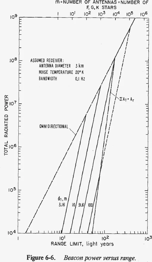
Beacons. A single directive beacon visiting stars in turn replaces by , so with equal effort at both ends no matter how hard both races try (eqs. 20–21). Pointing one antenna at each of stars works up to about 1000–2500 stars, 70 to 100 light-years, but the total power for directive beacons grows as the fifth power of range and eventually meets the omnidirectional line (Fig. 6-6). Long-range beacons will be omnidirectional and high powered (p. 61).
If the efficacy of a beacon–receiver pair is proportional to and every race minimises the total system cost (p. 61)
= cost per unit transmitter power capacity, taken as 2000 dollars/kW (300 dollars/kW nuclear plant plus 1200 dollars/kW conversion to monochromatic microwaves, rounded up); = cost per unit antenna area.
Spending 4 billion dollars on antennas therefore implies beacons of about 2000 MW, and the report expects beacon powers in excess of 1000 MW. Beacons would also transmit continuously, be extremely monochromatic, probably be circularly polarized, and carry information (pp. 61–62). Omnidirectional laser beacons fare poorly: at 1.06 μ, W reaches only 0.07 light-years, against 1360 light-years for a -W microwave beacon received by a 3-km array (Table 6-2, p. 63).
Likely beacon frequencies: the water holepp. 63–64
Six reasons favour the low end of the microwave window: smaller Doppler shifts, looser stability requirements, more collecting area for the narrowest usable beam, cheaper collecting surface, lower power densities in transmitters, and freedom from oxygen and water absorption. That points to roughly 1 to 3 GHz, still far too wide to comb into 1-Hz channels (p. 63).
Cocconi and Morrison had proposed the hydrogen line, and Project Ozma listened there for about 400 hours in 1960 to τ Ceti and ε Eridani. But transmitting and receiving on one natural frequency means self-jamming. What is wanted is a natural contact band, many times wider than the Doppler spread but narrow enough to search half of it at once, free of strong lines and not below the hydrogen line. The band from hydrogen (1420 MHz) to the lowest hydroxyl line (1662 MHz), less 10–20 MHz guard bands, leaves about 200 MHz of clear band (p. 64).
Where shall we meet? At the water hole, of course!Chapter 6, p. 64
Semantics and anticryptographypp. 64–65
Once a signal is found, the sender will have tried to make decoding easy, the reverse of cryptography. Drake and Oliver suggested pictorial messages: a repeated sequence whose length is the square of a prime invites arrangement as a raster of lines of bits. Compared with acquisition, all else is easy (pp. 64–65).
7. The Cyclops Systempp. 67–75
Chapter 7 condenses the design. Detecting coherent signals of intelligent origin seems to need 7 to 20 km² of collecting area, a clear aperture of 3 to 5 km. With the uncertainty in that figure perhaps a factor of ten either way, a phased array that can be expanded is preferred to any single antenna (p. 67).
The antenna array and system facilitiespp. 67–68
Each element is steered mechanically to about 10 arc-seconds; the final array beam, of an arc-second or less, is steered electrically by phase and delay. If element cost grows as the th power of diameter, the optimum makes structure cost times the fixed cost per element; the study found very near 2, so the elements are the largest fully steerable dishes yet built, 100 m in diameter, on azimuth–elevation mounts (p. 67).
Elements sit about three diameters apart to avoid shadowing at low elevation, in a roughly circular hexagonal lattice. An initial array of 100 or fewer elements (about 1 km clear aperture) would grow at the periphery, or be spread over the full area and filled in. From the air the final system would be a central headquarters amid an orchard of 1000 to perhaps 2500 antennas, 10 km to 10 miles across, linked by service tunnels carrying power, control, standard frequencies and the IF cables (p. 68).
Sky coverage and site selectionpp. 68–69
Noise and shadowing limit observation to elevations above about 20°. At 33° latitude that still covers 80 percent of the sky, against 94 percent at the equator (Fig. 7-1). The site should be geologically stable, dry, calm, large and flat, and remote from habitation and air routes; a remote site in the south-western United States is indicated, and the VLA siting study is pertinent (pp. 68–69).
Receiver system, IF transmission, IF delay, and control and monitoringpp. 69–71
The receivers cover 0.5 to 3 GHz, the low end of the window, using heterodyne conversion at each antenna. Local oscillators are synthesized at each antenna from two standard frequencies distributed from the centre, with phase errors of only a few degrees at 10 GHz. Halving receiver noise is worth doubling antenna area, so the front end is cooled up-converters followed by a fixed-frequency maser, about 20 K; bands change by commanding a new pump frequency. Both polarizations are received (p. 69).
The two 100-MHz IF bands go back on one coaxial cable per antenna, placed symmetrically about a pilot tone and inverted in frequency at the quarter and three-quarter points, so every band edge sees the same mix of frequencies and the cable loss is almost flat; holding the pilot's phase also measures and removes cable delay changes (p. 70). Delays of up to about 50 μs, held to ±1/8 ns, come from stripline, coax and acoustic surface-wave lines, temperature-servoed against the pilot. All antennas normally point and tune together; time-multiplexed control allows independent sub-arrays (p. 70).
Combing the spectrum for signs of lifepp. 71–72
The signal processor is what makes Cyclops a search instrument. Each band is recorded as a raster on film and Fourier-transformed by a lens into its power spectrum, so a coherent signal becomes a needle. Successive spectra are then added with a range of offsets to follow any plausible drift; in the addition that matches the drift, the needle builds into a spike above the noise (p. 71).
Recording 200 MHz for about 1000 s gives 100 spectra at 0.1 Hz resolution. Added about 400 ways, they yield some 100 independent composite signals of Nyquist intervals per polarization: tests per observation. For a 20 percent false-alarm chance per observation, each test needs about . A signal at unity signal-to-noise in 0.1 Hz, dB relative to the whole 200-MHz band, is then missed half the time; 2 dB more brings misses to 1 percent (pp. 71–72).
Imaging the radio sky and the auxiliary optical systempp. 72–73
Because each element's IF signal returns independently, elements can form simultaneous beams. The proposed imager re-radiates the signals at their original frequency from a scaled model of the array, 20 m across, onto an image array 40 to 120 m away, inside an anechoic, shielded building about 75 × 75 × 550 ft. Several optical telescopes, including a 1-m Schmidt to survey for target stars, would complete the site (pp. 72–73).
Range capabilityp. 73
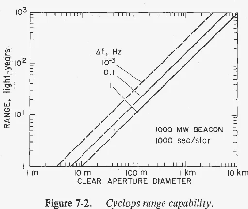
For a 1000-MW beacon and 1000 s per star, the range with 1-Hz resolution is simply 100 light-years per kilometer of antenna diameter; 0.1-Hz resolution adds a factor of 1.6 (p. 73).
The cost of Cyclopspp. 73–74
Costs are plotted against clear aperture, about one-third of the physical array diameter. Tunnels, receivers, IF delay and imager scale with the number of elements; IF transmission scales as its 3/2 power. The signal detector is a fixed 160 million dollars (optical analyzers with time-bandwidth product and 1000 s per star), or 45 million dollars with and 100 s; engineering is a rough 100 million dollars, buildings 10 million dollars and the optical system 2 million dollars (p. 73).
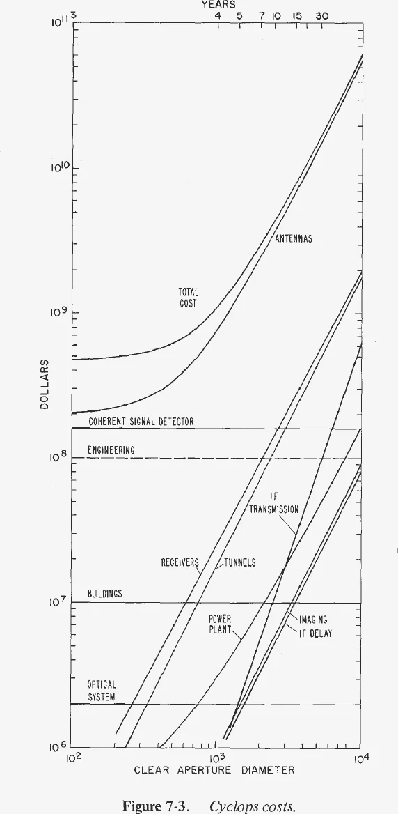
Above a few hundred metres of aperture the antenna structures dominate: here is where creative innovation would really pay. Lowering the elements' top frequency from 10 to 3 GHz might halve their cost (pp. 73–74).
A comparison of the Cyclops and Ozma systemspp. 74–75
| Parameter | Symbol | Ozma | Cyclops |
|---|---|---|---|
| Antenna diameter | d | 26 m | 3160 m |
| Antenna efficiency | η | 0.5 | 0.8 |
| System noise temperature | T | 350 K | 20 K |
| Resolved bandwidth | Δf | 100 Hz | 0.1 Hz |
| Integrating time | τ | 100 s | 10 s |
| Instantaneous bandwidth | B | 100 Hz | 200 MHz |
Sensitivity taken proportional to ; range goes as its square root and searchable volume as range cubed.
A signal Ozma could have seen at τ Ceti or ε Eridani, 10–11 light-years away, Cyclops could see at 20,000 light-years, or a signal 1/400 as strong at 1000 light-years. Those stars would have needed about W of effective radiated power to move Ozma's pens; Cyclops would detect 2.5 MW. Cyclops also searches two million times the band, for a spectrum search rate 200,000 times faster (pp. 74–75).
Confusion limitation. Going from one 100-m dish to 1000 dishes over 10 km raises sensitivity -fold but resolving power -fold, so the array becomes confusion-limited only if the log N–log S curve is steeper than , which the authors consider unlikely (p. 75).
8. Antenna Elementspp. 77–85
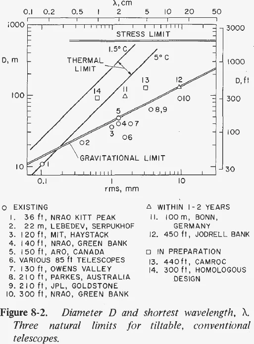
The tentative specifications were a total equivalent diameter of up to 10 km, 500 MHz to 10 GHz, a minimum elevation of 20°, operation at 10 GHz in winds to 20 mph and survival to at least 100 mph (p. 77). Fixed spherical dishes, troughs and tilting flats were considered, and a 3-km space dish rejected as beyond present or near-future technology. The choice is a conventional steerable dish on a wheel-and-track azimuth–elevation mount (pp. 77–78).
Surface tolerance. A normally distributed surface error reduces the gain by (p. 79)
Allowing at 10 GHz sets mm, with high efficiency over the primary range below 3 GHz.
Optimum sizing. Following Drake, the cost per element is , with the fixed per-element cost of receivers, control and IF. For a total effective area the total cost and its minimum are (p. 80)
If there is no optimum and the largest buildable dish is best.
Earlier studies had found exponents of about 2.78 to 3. Correcting seven recent designs to 1970 U.S. dollars (Table 8-2), the Cyclops group found dollars with in feet, which rounds to (pp. 81–82)
= equivalent clear-aperture diameter of the array; = cost reduction factor from mass production; = aperture efficiency of the elements ( expected).
The exponent of 2 is explained by labour: of roughly 10 million dollars for the Bonn dish, raw material at 10 cents a pound is only 640,000 dollars (pp. 82–83). Industry discussions put mass-production savings at 20 to 40 percent; others suggested 60 to 70 percent (p. 84).
| Equivalent diameter, km | R = 0.7, billion dollars | R = 0.4†, billion dollars |
|---|---|---|
| 1 | 1 | 0.78 |
| 2 | 4 | 2.5 |
| 3 | 9 | 5.2 |
| 5 | 25 | 14 |
† Includes 200 million dollars of tooling. For an ultimate 5-km system the structures fall in the range of 10 to 25 billion dollars, and the report names a large study to reduce and refine this figure the first order of business (p. 84).
9. The Receiver Systempp. 87–105
The design goals are high aperture efficiency (10 percent more could save a billion dollars), the lowest possible noise, wide instantaneous bandwidth, rapid remote band switching, any polarization, and automatic phasing, calibration and fault detection (p. 87). Six bands, each covering a 1.35-to-1 range, span 0.5 to 3 GHz (p. 88):
| Band | Range, GHz | Coverage, MHz |
|---|---|---|
| 1 | 0.5 – 0.675 | 175 |
| 2 | 0.675 – 0.91 | 235 |
| 3 | 0.91 – 1.23 | 320 |
| 4 | 1.23 – 1.66 | 430 |
| 5 | 1.66 – 2.24 | 580 |
| 6 | 2.24 – 3.02 | 780 |
Each band has a circularly symmetric feedhorn and two up-converters, one per polarization, cooled to 20 K and feeding 10-GHz masers at 4 K. From two received polarizations the centre can form six (V, H, the two 45° linears and both circulars): processing all six limits the loss for an unknown polarization to 1 dB, against 3 dB with four, and processing is far cheaper than antenna (p. 88).
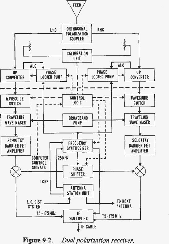
Cassegrain optics put the feed cluster in the secondary's shadow, aim feed spillover at the sky rather than the hot ground, and allow sharper-edged illumination; Sonine illumination patterns give efficiency , and illumination efficiencies near 90 percent are considered realizable (pp. 89–91). Estimated system noise runs from about 40 K at 500 MHz to 24 K at 3 GHz, with a minimum near 20 K around 1.5 GHz (p. 96).
A hydrogen maser, about 30 times better than rubidium and 500 times better than cesium at 100-s averaging, is the frequency standard; three are recommended so that a disagreement can be resolved (p. 96). Receiver electronics are estimated at 300,000 dollars per antenna in small quantities, perhaps 200,000 dollars in production (Table 9-2, p. 104).
10. Transmission and Controlpp. 107–122
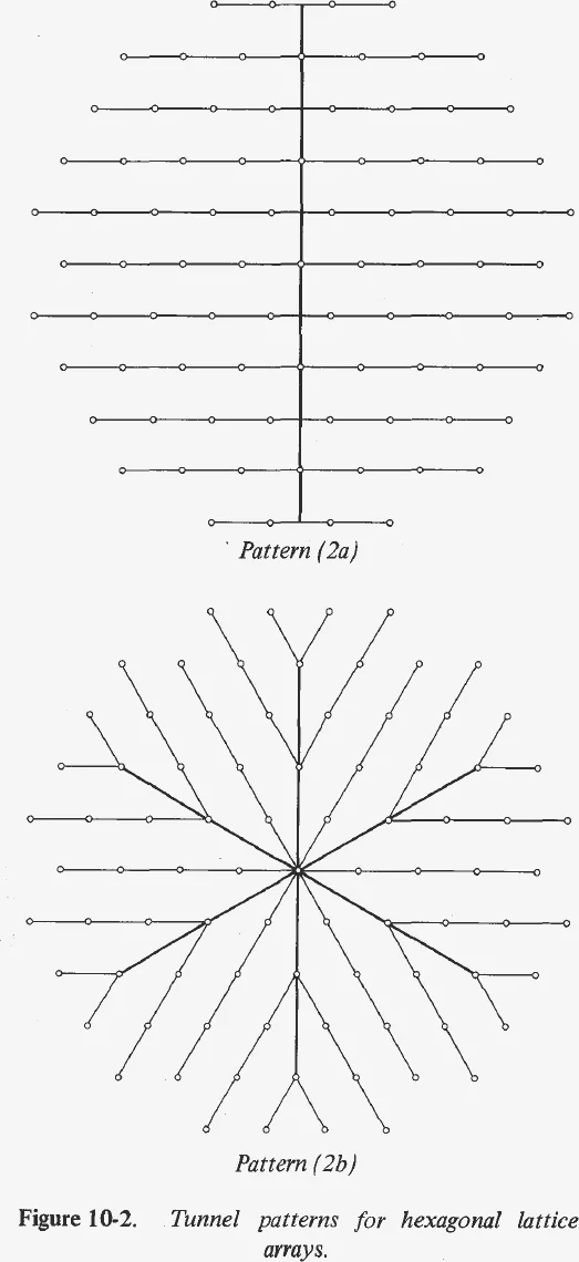
To avoid shadowing down to elevation , antennas sit apart (eq. 1), about three diameters at 20°. Since the array will grow for 10 to 20 years, all services run in tunnels that are extended as it grows; tunnels 8 ft across cost about 570 dollars/m, giving (eq. 4, pp. 107–109).
Coaxial cable is chosen for IF transmission over circular waveguide, free-space and guided lasers, optical fibres and microwave links, which were less developed in 1971 (pp. 109–110). The longest IF cables in a 10-km array are about 6 km; a 10 °C swing changes their length by about a metre, hence the pilot-tone compensation (p. 110). A modest computer suffices for control: 32K words of memory and a system cost under 120,000, dollars duplicated for safety (p. 121).
| 100-m antennas | Equivalent aperture, km | Peak, MW | Average, MW | Cost, million dollars |
|---|---|---|---|---|
| 100 | 1 | 4 | 2.2 | 2.4 |
| 200 | 1.4 | 7 | 3.4 | 4.2 |
| 500 | 2.2 | 16 | 7 | 10 |
| 1000 | 3.16 | 31 | 12 | 20 |
| 2000 | 4.4 | 61 | 25 | 36 |
Includes the control centre and a community of about one person per antenna; nuclear generation assumed at 300 dollars/kW plus 300 dollars/kW for buried distribution (pp. 121–122).
11. Signal Processingpp. 123–152
The detection of narrow band signalspp. 123–126
The aim is a receiver with to channels of 1 or 0.1 Hz watching the whole 100-MHz IF band at once (p. 123). Alternatives are examined first. Total-power detection of a signal that doubles the noise in one 1-Hz channel would need samples, about three years of integration. Cross-power detection between two half-arrays also correlates the sky background and star noise and halves the area. A Golay detector carries no more information than a simple square-law detector, and a scanning analyzer wastes all but of the data (pp. 123–125).
A hard-wired fast Fourier transform of points takes s (eq. 5). For real-time 1-Hz resolution one unit handles about 11,000 Hz, so two 100-MHz bands would need some 18,000 units at about 4.5 billion dollars, which leads to the optical approach (p. 126).
The optical spectrum analyzerpp. 126–129
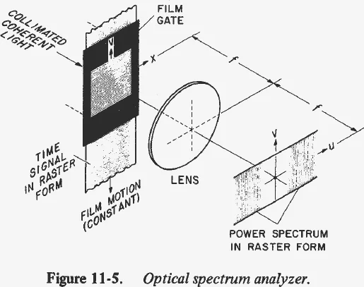
The IF signal, biased positive, modulates a laser that writes a raster on moving film. In the analyzer's gate a lens transforms the film's transmission into its power spectrum, which appears in the back focal plane, itself in raster form: each line spans a band equal to the scanning frequency. A gate holding a signal duration resolves (p. 128)
= time-bandwidth product. had been achieved and was believed possible.
| Δf | Na (N = 10⁶) | Million dollars | Na (N = 10⁷) | Million dollars |
|---|---|---|---|---|
| 10 Hz | 20 | 2 | 2 | 0.24 |
| 1 Hz | 200 | 20 | 20 | 2.4 |
| 0.1 Hz | 2000 | 200 | 200 | 24 |
Film use for 200 MHz at 3000 lines/cm is about 22 cm²/s, roughly 47 dollars an hour on 35-mm stock (p. 129).
Power spectrum processingpp. 129–136
A weak drifting signal is invisible in any one spectrum but appears as a slanting trace in a stack of them, like the pulsar record of Fig. 11-7. The spectra are scanned by a high-resolution vidicon, stored on head-per-track magnetic disks (about 120,000 dollars per second of observing, so 120 million dollars for 1000 s), then played back together down tapped video delay lines whose taps, in slanting rows, form the composite signals (pp. 130–133).
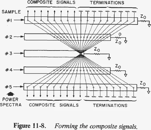
If the true drift differs from the nearest composite by resolution intervals across the stack, the detection efficiency is (p. 133)
is down 1 dB at ; keeping () for drifts of up to one interval per spectrum needs composite signals from spectra.
Costing the storage, analyzers, delay lines, taps and detectors (eq. 21) for 100-MHz channels and 1000 s gives 264 million dollars for 1-Hz channels with analyzers, 480 million dollars for 0.1 Hz, and 135 dollars and 158 million dollars with : from 125 dollars to 500 million dollars in round numbers (pp. 135–136). The authors present this as a sort of existence proof, expecting better or cheaper methods (p. 136).
Statistics of the detection processpp. 136–140
The analyzer's output brightness has the statistics of a square-law detector. If is the average of samples, normalised so that the mean noise is 1, then with noise alone (Appendix D, p. 137)
= probability per datum that noise alone exceeds the threshold .
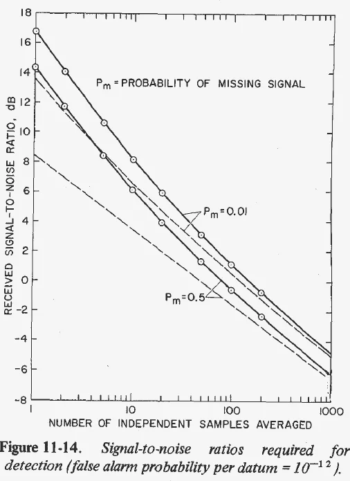
An observation holds independent data for MHz and s (eq. 27). If false alarms may lengthen the search by , then ; the report uses (eqs. 28–30, pp. 137–138). With signal-to-noise ratio in one resolution bin, follows
= modified Bessel function of the first kind. The miss probability is the integral of below , found numerically on an HP 9100B calculator (p. 138).
After 80 averages a unity (0 dB) signal is missed half the time at a false-alarm rate; after 150, only 1 percent of the time; and beyond two decibels take the miss rate from 50 to 1 percent. With Hz and , a coherent signal 90 dB below the total noise power in the 100-MHz band can be found (pp. 138–139).
Low frequency time anomaly detector and Drake ensemble signal detectionpp. 140–141
For pulsed or swept signals such as pulsars, one analyzer can cover the whole 100-MHz band at 100-Hz resolution and 0.01-s integration, watched by vidicon, for perhaps 300,000 dollars (p. 140). Drake's ensemble method cross-correlates two successive power spectra to detect many weak narrow-band signals collectively. Its gain over a conventional detector depends on the fraction of occupied channels: about 0.70 for Earth's UHF television band and 1.25 for the FM band; it is recommended as an inexpensive addition (pp. 140–141).
Wide band imaging of the radio skypp. 141–152
With 1000 dishes over 10 km at 10 cm there are about resolvable directions: 5000 years to map the sky at one second per point with one beam, or 5 years with 1000 simultaneous beams (p. 142). Radiative imaging must be done at, or near, the received frequency to avoid lateral chromatic aberration (eqs. 52–53). Delay-line, acoustic and optical imagers are compared; a microwave imager with plane signal and image arrays focused by paraboloidal delay is preferred, at about 9.2 million dollars including its shielded building (pp. 143–151).
Undesired signals. Unlike radio astronomy, Cyclops must work outside protected bands. UHF television would overload any reasonable receiver, low-power stations would be detectable for several hundred miles, and any flying object out to lunar distances. Options include a concentric secondary beam to subtract interference, a catalogue of known transmitters, or a quiet zone around the array (p. 152).
12. Cyclops as a Beaconpp. 153–154
With a 100-kW transmitter on each of 1000 dishes (100 MW total, perhaps 300 MW of input power), the whole array aimed at one star at 1.5 GHz radiates an effective W; each element used alone, W (p. 153). A 10-m antenna with a 10-kHz bandwidth could detect the full array at about 80 light-years, and a 1-Hz receiver on a simple dipole at 50 light-years. Used one star per dish, a 100-m, 1-Hz search receiver could still detect it at 80 light-years (pp. 153–154).
Parallel searching of many stars is ruled out by the cost of replicated data processing, so the search stays serial. The array can, and probably should, illuminate stars closer than 100 light-years for part of the search phase, and provides a built-in response system for any signal found (p. 154).
13. Search Strategypp. 155–164
The goal is to maximise the probability of contact after any search time. With an a priori probability depending on spectral class and range, the strategy is to work down a list in order of decreasing , revised as the array grows (eqs. 1–2, p. 155). The real obstacle is the list: distances are known for only a few hundred target stars, under a thousandth of those needed out to 1000 light-years (p. 156).
Parallax works only to about 50 parsecs, and proper motion is unreliable. Distance from absolute magnitude, pc (eq. 3), requires knowing that a star is on the main sequence. UBV photometry confuses giants with late-G and K dwarfs and suffers from reddening; objective-prism spectroscopy to magnitude 16 would mean 20 million spectra, about 1000 man-years. The proposal is an automated photoelectric survey of star fields in several spectral bands, refined by several smaller telescopes (pp. 157–161).
The search falls into four phases: a pre-operational phase compiling the target list; the construction years, at perhaps 100 antennas a year over 10 to 25 years, with range growing as the square root of time and stars searched as the 3/2 power (Fig. 13-4 assumes 15,000 stars a year at 2000 s each); a total search with the complete system out to 1000 light-years; and, if nothing is found, a long-term effort including a possible long-range beacon (pp. 161–162). An area search of one or two degrees about the galactic centre, and its antipode, is also recommended, after a suggestion of Joshua Lederberg (p. 163).
14. Cyclops as a Research Toolpp. 165–168
A 3-km equivalent Cyclops would collect m², 2200 times the JPL 210-ft antenna and 6700 times Haystack, with about 1 arc-second resolution at 3 cm (p. 165). Deep-space probes at Uranus could return what Mars probes did, and any experiment possible with the 210-ft antenna could reach 47 times as far. As a radar receiver it would extend planetary radar range 7 to 9 times, or 47 to 81 times with transmitters on every element, enough to map Pluto (pp. 165–166).
For radio astronomy it would offer source counts to the cosmological horizon, 21-cm hydrogen and molecular-line spectroscopy at 1-Hz resolution over 100 MHz in real time, most of the galaxy's estimated to pulsars and those of the Virgo cluster, and radio emission from many nearby normal stars. Combined with a distant 30-m dish it would form a very powerful interferometer (pp. 166–167). The authors suggest using no more than 10 percent of Cyclops's time this way, and ask that other instruments not be planned around Cyclops until it is funded (p. 168).
15. Conclusions and Recommendationspp. 169–172
The chapter restates seven premises, among them that planetary systems are the rule, that F- to K-type main-sequence stars live long enough for evolution, and that the longevity of technological civilizations is unknown within orders of magnitudes (p. 169). Fifteen conclusions follow (pp. 170–171), the consensus of the System Design Group; among them:
- Looking for and sending signals is vastly cheaper than contact by spaceship or probe, by physical law rather than present technology.
- The uncertainty in distance between civilizations argues for an expandable system.
- Microwaves are the best means, and the best part is the low end of the window, about 1 to 2 or 3 GHz.
- The quiet band between hydrogen (1420 MHz) and hydroxyl (1662 MHz), the water hole, seems especially marked for contact.
- Phased arrays of 100 km² or more are technologically feasible in the 1–3 GHz region.
- Long-range beacons will probably be omnidirectional and very high powered (more than 10⁹ W), circularly polarized and highly monochromatic.
- The Cyclops processor searches 100 MHz at once with 0.1-Hz resolution, a billion channels; widening to 200 MHz would cover the whole water hole.
- An effective system costs on the order of 6 to 10 billion dollars over 10 to 15 years, mostly in antenna structures.
- The search may take years, decades or centuries, and needs long-term commitment.
- International cooperation should be encouraged by complete dissemination of information.
The ten recommendations include making the search an ongoing part of NASA's programme with its own budget and an office of research and development; protecting the water hole, 1.4 to 1.7 GHz, through the FCC and international agencies; an advisory committee perhaps through the National Academies to oversee 3 to 5 years of preliminary studies; open liaison abroad with no classified information; and public reporting and education (pp. 171–172).
Appendices A–R (pp. 173–243) give astronomical data, an essay on supercivilizations and cultural longevity, and the supporting analyses: optimum detection, square-law detection theory, base and back-up structures, polarization, Cassegrain geometry, local-oscillator phasing, cable dispersion and lengths, phasing and delay, calibration, the optical analyzer, lumped delay lines, detection-statistics curves, and the radio visibility of normal stars.
Assumptions and open questions
Key assumptions
- Other civilizations communicate with electromagnetic waves and favour the same low end of the microwave window, and plausibly the water hole, for the same physical reasons (Chs. 5–6).
- The most detectable signals are intentional, continuous, highly monochromatic and probably circularly polarized beacons of about 1000 MW or more; leakage is detectable only from nearby stars (pp. 59–62).
- Target stars are F, G and K main-sequence stars within about 1000 light-years, about 1.7 million of them from Allen's density and the 850-light-year scale height (pp. 53–55).
- The reference performance assumes a 20 K system, 1000 s per star, a false-alarm rate of 10⁻¹² per datum, and drifts of at most one resolution interval per spectrum (pp. 73, 134–138).
- Antenna structure cost scales as diameter squared (1156 d² dollars, 1970 prices) over 25–150 m, so the largest steerable dish, 100 m, is chosen; mass production saves 30 to 60 percent (pp. 82–84).
- Subsystem designs use 1971 technology: film-based optical spectrum analysis, analog disk storage, coaxial IF cables and cooled up-converters with masers (Chs. 9–11).
Where further work would help
- Antenna cost law. The whole system cost rests on the exponent fitted to seven designs and on the mass-production factor. The report itself calls a large study of element cost the first order of business (p. 84); a wider set of designs would show how sensitive the optimum element size and total cost are to that exponent.
- Beacon power and duty. Range scales with the square root of effective radiated power, and the 1000-MW figure comes from a cost-balancing argument (eqs. 22–23). How the search time changes across a wider range of assumed powers, duty cycles and drift rates would bound how far the 1000-light-year design target can be relied on.
- Signal processing. The detection statistics assume independent spectra, a rectangular analyzer gate and a fixed drift per observation. Testing with real interference, non-constant drift and the continuous-averaging variant (about 1 dB better, p. 139) would show how the 90-dB sensitivity holds up in practice.
- Target list. The search order depends on knowing spectral class and distance for about a million stars, and the report notes that no rapid method yet existed (p. 160). The effect of an incomplete or diluted list on the time to contact is not quantified.
- Terrestrial interference. Chapter 11 estimates that television and aircraft would be strongly detectable (p. 152). How much of the 0.5–3 GHz range, and of the water hole itself, remains usable at a real site would set the practical bandwidth.
- Sky and noise models. The sky-noise curves of Fig. 5-2 are described as approximate and elevation dependent (p. 41), and the range figures take the receiver at 20 K; site measurements would show how far the quoted ranges extrapolate to low elevations and the band edges.
What happened next
- 1973
Oliver spends more than a year editing the report, which is published in 1973; 10,000 copies are printed. Billingham later notes that its picture of the full 1,000-dish array, with its price of 6–10 billion dollars, fed a lasting belief that the full array was needed to detect anyone, although it was to be built and used in stages.
- 1975
Ames holds a series of SETI Science Workshops chaired by Philip Morrison through 1975 and 1976. At the December 1975 meeting the group adopts John Wolfe's name, the Search for Extraterrestrial Intelligence: SETI.
- 1977
The workshops' report, NASA SP-419, recommends starting a SETI programme with existing telescopes. It records that a JPL review found the Cyclops report correct in its major technological conclusions, and that million-channel solid-state Fourier analyzers could now replace the optical processor.
- 1978
Senator William Proxmire gives the programme a Golden Fleece award. In 1981 his amendment removes all 1982 funding; NASA restores SETI to its 1983 budget request, and Carl Sagan and others persuade Proxmire not to oppose it again.
- 1992
Oct 12: NASA inaugurates the High Resolution Microwave Survey, a targeted search at Arecibo and a sky survey at Goldstone, with a 1992 budget of 17.5 million dollars.
- 1993
Senator Richard Bryan's amendment eliminates the programme; NASA's SETI office closes in March 1994, after total SETI spending of just under 78 million dollars. Billingham writes that Cyclops has been gradually superseded by the SETI Institute's Allen Telescope Array and the proposed Square Kilometre Array.
Sources
- Oliver & Billingham, Project Cyclops: A Design Study of a System for Detecting Extraterrestrial Intelligent Life (NASA CR-114445)
- J. Billingham, "SETI: The NASA Years," in D. A. Vakoch, ed., Archaeology, Anthropology, and Interstellar Communication (NASA SP-2013-4413), pp. 1–21 · Cyclops pp. 4–6; workshops pp. 7–8; Proxmire pp. 10–11; HRMS and cancellation pp. 18–21
- P. Morrison, J. Billingham & J. Wolfe, eds., The Search for Extraterrestrial Intelligence (NASA SP-419, 1977) · Preface and Section I conclusions
- NASA History: NASA and the Search for Extraterrestrial Intelligence
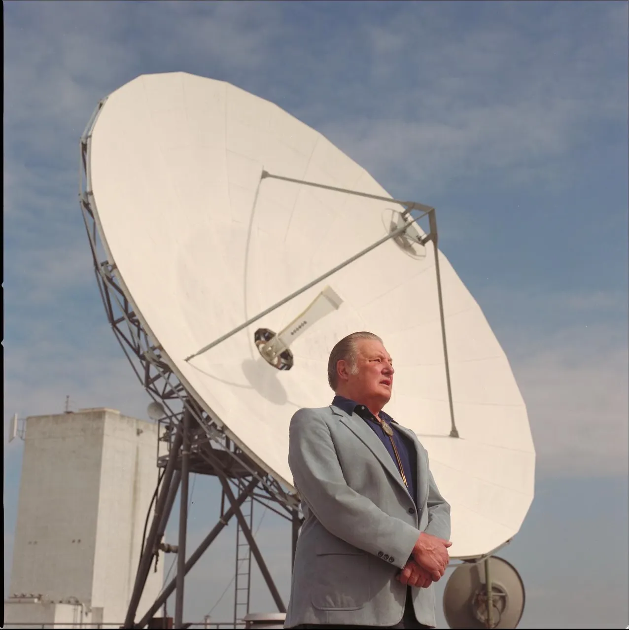
- NASA Image Library: Dr Bernard Oliver, Ames SETI Office, 1986